Expectation and Sample Mean
For a certain distribution  , we know the expectation. If we get a sample of , which we call it
  , we are also able to calculate the empirical average or mean of the sample,
  .
.
Contents
What's the relationship between empirical mean and theoretical expectation?
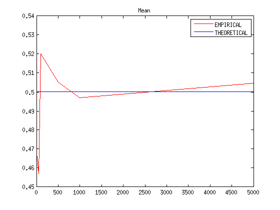
Uniform distribution example
 ;
;
alpha1 = 0;
beta1 = 1;
Compute THEORETICAL values;
mean1 = (beta1 - alpha1) / 2;
Compute empirical values;
sizes = [5,10,50,100,500,1000,5000]; % For different sampling sizes;
nS = length(sizes);
mean2 = zeros(nS,1);
variance2 = zeros(nS,1);
for sizeIndex = 1:nS
    aSize = sizes(sizeIndex);
    ys = unifrnd(alpha1, beta1,[aSize,1]);
    mean2(sizeIndex) = mean(ys);
    variance2(sizeIndex) = var(ys);
end
fig1a = figure;
xlim([min(sizes) max(sizes)]);
ylim([0, max(mean2)]);
plot(sizes,mean2, '-r');
hold on;
plot(sizes,repmat(mean1,1,nS),'-b');
legend('EMPIRICAL','THEORETICAL');
title('Mean');
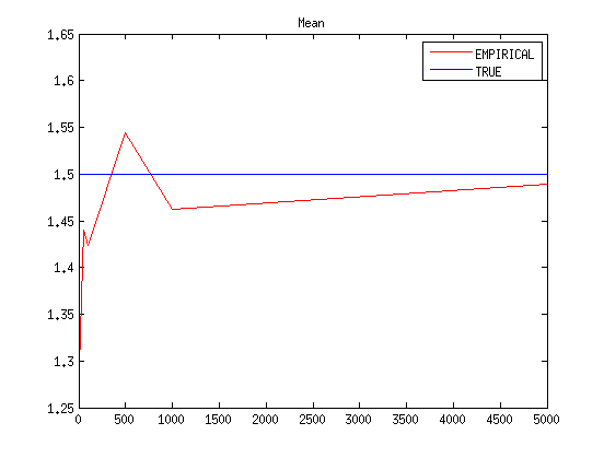
Pareto distribution example
Let's do the same for  ;
;
alpha1 = 3;
k1 = 1/alpha1;
sigma1 = 1/alpha1;
theta1 = 1;
Compute THEORETICAL values;
mean1 = alpha1/ ( alpha1 - 1);
Compute empirical values;
rep = 100;
sizes = [5,10,50,100,500,1000,5000];
nS = length(sizes);
mean2 = zeros(nS,1);
for sizeIndex = 1:nS
    aSize = sizes(sizeIndex);
    aMean = 0;
    ys = gprnd(k1,sigma1,theta1,[aSize,1]);
    mean2(sizeIndex) = mean(ys);
    variance2(sizeIndex) = var(ys);
end
fig1a = figure;
xlim([min(sizes) max(sizes)]);
ylim([0, max(mean2)]);
plot(sizes,mean2, '-r');
hold on;
plot(sizes,repmat(mean1,1,nS),'-b');
legend('EMPIRICAL','TRUE');
title('Mean');