Lab 4, Chapter 6 - Simulation. (Due on 09:00 PM, Mar 13, 2015)

Random number generator is based on the simulation theory. Simulation is to accosiate two distributions, specifically speaking, associate the probability of two events defined on two random variables X and Y. X, Y can be either discrete, or continuouse.

Generate random numbers for random variable $X\sim Bin(3, 0.5)$
Generate random numbers for random variable $X \sim Exp(2)$
Assignments

Generate random numbers for random variable $X\sim Bin(3, 0.5)$

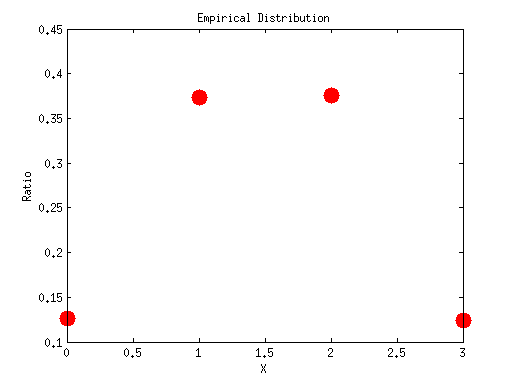
A. Generate 10000 numbers directly from binornd() function

numOfPoints = 10^5;
n = 3;
p = 0.5;
xs = binornd(n, 0.5, [1, numOfPoints]);
max(xs);
min(xs);

Now let's draw the empirical distribution of the random numbers. Let's count the number of random numbers we get for values {0, 1, 2, 3}, respectively.

valueCounts = hist(xs, 0:1:3);
valueRatios = valueCounts / numOfPoints;
plot(0:1:3, valueRatios,'r.', 'MarkerSize', 40);
title('Empirical Distribution');
xlabel('X');
ylabel('Ratio');

B. Generate 10000 binormial numbers by simulation using $U\sim U(0,1)$ distribution. According to the table of Homework Q1.

$P(X = 0) = P(0 \leq U < 1/8) = 1/8, P(X = 1) = P(1/8 \leq U < 4/8) = 3/8$ ,

$P(X = 2) = P(4/8 \leq U < 7/8) = 3/8, P(X = 3) = P(7/8 \leq U < 1) = 1/8$ . So the code would be,

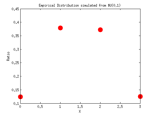
1) if we get a random number u within [0, 1/8), we assume we get the a 0 for X,

2) else if we get a random number u within [1/8, 4/8), we assume we get a 1 for X,

3) else if we get a random number u within [4/8, 7/8), we assume we get a 2 for X,

4) else if we get a random number u within [7/8,1) we assume we get a 3 for X.

xs_simulated = [];
us = unifrnd(0,1, [1,numOfPoints]);
for i = 1:numOfPoints
    u = us(i);
    if( u >= 0 && u < 1/8)
        x = 0;
    elseif( u >= 1/8 && u < 4/8 )
        x = 1;
    elseif( u >= 4/8 && u < 7/8 )
        x = 2;
    elseif( u>= 7/8 && u < 1 )
        x = 3;
    end
    xs_simulated(i) = x;
end

Plot the empirical distribution for xs_simulated

valueCounts = hist(xs_simulated, 0:3);
valueRatios = valueCounts / numOfPoints;
plot(0:3, valueRatios,'r.', 'MarkerSize', 40);
title('Empirical Distribution simulated from $U(0,1)');
xlabel('X');
ylabel('Ratio');

Generate random numbers for random variable $X \sim Exp(2)$

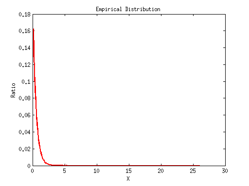
A. Generate 10000 numbers directly from exprnd() function

numOfPoints = 10^5;
lambda = 2;
xs = exprnd(1/lambda, [1, numOfPoints]);  % Pay attention exprnd() takes a parameter mu, which is 1/lambda.
max(xs);
min(xs);

Now we can draw the empirical distribution for xs. Since xs can be [0, infinity), we will set the stepsize a little smaller, but not too small.

valueCounts = hist(xs, 0:0.1:26);
valueRatios = valueCounts / numOfPoints;
plot(0:0.1:26, valueRatios,'r-','LineWidth', 2);
title('Empirical Distribution');
xlabel('X');
ylabel('Ratio');

% *B. Generate 10000 numbers by simulation using $U\sim U(0,1)$ distribution.*

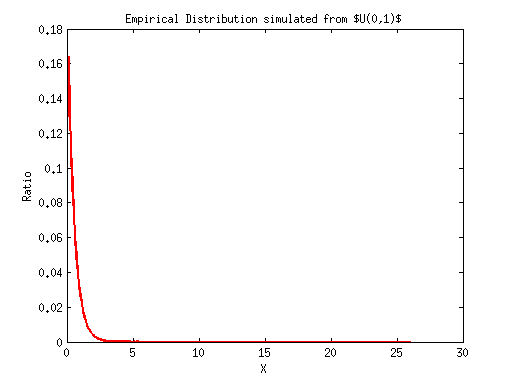
According to the formula in Homework 5 Q3. The simulation rule is:

$x = -\frac{1}{2}ln(1-u)$ . So the pseducode shall be:

For any random number u we get, let $~~~x = -\frac{1}{2}ln(1-u)$ .

xs_simulated = [];
us = unifrnd(0,1, [1,numOfPoints]);
for i = 1:numOfPoints
    u = us(i);
    x = -1/2 * log(1 - u);
    xs_simulated(i) = x;
end
valueCounts = hist(xs_simulated, 0:0.1:26);
valueRatios = valueCounts / numOfPoints;
plot(0:0.1:26, valueRatios,'r-','LineWidth', 2);
title('Empirical Distribution simulated from $U(0,1)$');
xlabel('X');
ylabel('Ratio');

Assignments

Question1 . Generate 100000 random numbers for $X \sim Geo(0.5)$ distribution.

a). Generate using Matlab built-in function geornd().

b). Generate by simulation using $U \sim U(0,1)$ distribution.

c). Draw the empirical distribution for the numbers generated from a) or b). Do they look similar?

Question2 . Generate 100000 random numbers for $X \sim Par(3)$ distribution.

a). Generate using Matlab built-in function gprnd() . (Hint: To get Par(3), with $\alpha = 3$ . You need to set the $k = 1/\alpha, sigma= 1/\alpha, theta = 1$ .)