Lab 3, Discrete, continouse distribution. SOLUTION (Due on 11:59 PM, Feb 17, 2015)

Assignments

Assignments

Here goes the assignments for Lab 3.

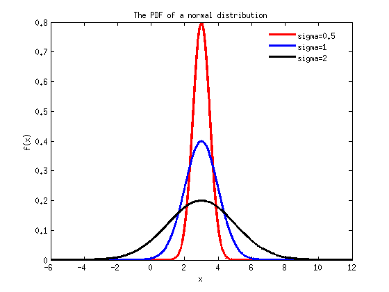
Question 1. Plot the PDF and CDF for normal distribution with fixed $\mu = 3$ and varying $\sigma = [0.5, 1, 2]$ . Draw your observations with two to three sentences.

mu=3;
sigma=[0.5 1 2];
xs=-6:0.0001:12;
linestyle={'r-','b-','k-'};

%plot the PDF of a normal distribution
fig1=figure;
for i=1:3
f=normpdf(xs,mu,sigma(i));
plot(xs,f,linestyle{i},'linewidth',3);
hold on;
end
title('The PDF of a normal distribution');
xlabel('x');ylabel('f(x)');
legend('sigma=0.5','sigma=1','sigma=2','location','best');
legend('boxoff');

plot the CDF of a normal distribution

fig2=figure;
for i=1:3
F=normcdf(xs,mu,sigma(i));
plot(xs,F,linestyle{i},'linewidth',3);
hold on;
end
title('The CDF of a normal distribution');
xlabel('x');ylabel('F(x)');ylim([-0.02 1.02]);
legend('sigma=0.5','sigma=1','sigma=2','location','best');
legend('boxoff')

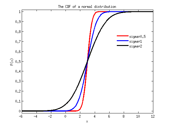
Observations: PDF: All three plots have the same median (mu, in this case 3). The smaller sigma is, the higher and narrower the peak in the middle of the plot (around x=3). CDF: The smaller sigma is, the steeper and closer to vertical the corresponding plot is. All three plots go through the same point at F(x) = 0.5 (which is the median).

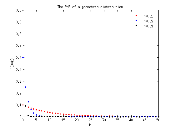
Question 2. Plot the PMF and CDF for geometric distribution with varying $p=[0.1, 0.5, 0.9]$ .

p=[0.1 0.5 0.9];
ks=0:50;

plot the PMF of a geometric distribution

fig3=figure;
linestyle={'r.','b.','k.'};
for i=1:3
P=geopdf(ks,p(i));
plot(ks,P,linestyle{i},'markersize',13.5);
hold on;
end
title('The PMF of a geometric distribution');
xlabel('k');ylabel('P(X=k)');
legend('p=0.1','p=0.5','p=0.9','location','best');
legend('boxoff');

%plot the CDF of a geometric distribution
fig4=figure;
linestyle={'r-','b-','k-'};
for i=1:3
F=geocdf(ks,p(i));
stairs(ks,F,linestyle{i},'linewidth',3);
hold on;
end
title('The CDF of a geometric distribution');
xlabel('x');ylabel('F(x)');ylim([-0.02 1.02]);
legend('p=0.1','p=0.5','p=0.9','location','best');
legend('boxoff');

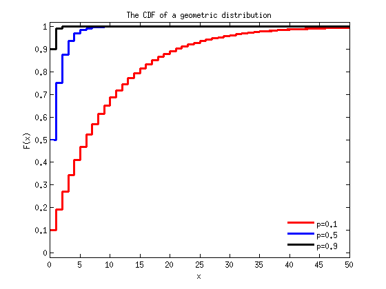
Observations: PMF: The larger p is, the more quickly f(x) approaches 0. CDF: The larger p is, the more quickly F(x) approaches 1.

Submission. Put all of your code, figures, writeups in a single document with .doc or .docx or .pdf format. Submit the document through blackboard. Attention, .txt format is not acceptable.

Lab 3, Discrete, continouse distribution. SOLUTION (Due on 11:59 PM, Feb 17, 2015)

Contents

Assignments