Lab 3, Discrete, continouse distribution. (Due on 11:59 PM, Feb 17, 2015)
Any distribution can be plotted with Matlab®. In Lab 3, we will show the impact of different controling parameters on several discrete and continouse distributions we learnt so far. All the distributions that are available in Matlab : http://www.mathworks.com/help/stats/binopdf.html
Contents
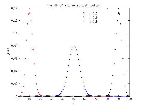
Plot the PMF of a binomial distribution by varying p;
Step 1. define neccessary variables(Matlab variables) to code for the binomial PMF formula  .
.
n = 100;            % the n parameter in the PMF.
p = [0.1, 0.5, 0.9];% the varying p parameter in the PMF.
ks = 0:100;          % the value X can take.
Step 2. In each iteration of the for loop, calculate the corresponding P according to the binomial PMF formula. Draw a PMF on a figure.
fig1 = figure;      % create a figure to draw on.
linestyle = {'r.', 'b.','k.'};
for i=1:3
    P = binopdf(ks,n,p(i));   % Directly call the binopdf() function to calculate P(X=k) returns a vector of probabilities with the same length as ks
    plot(ks, P, linestyle{i}, 'linewidth', 3); % .r means red dots. -r means red line.
    hold on; % hold on for other plotting.
end
title('The PMF of a binomial distribution');
xlabel('k');
ylabel('P(X=k)');
legend('p=0.1','p=0.5', 'p=0.9','Location','best');
legend('boxoff');
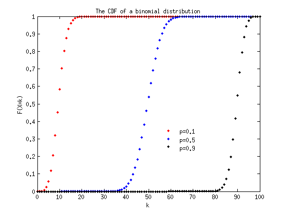
Plot the (Cumulative) Distribution Function of a binomial distribution by varying p;
Step 1. define neccessary variables(Matlab variables) would be used.
n = 100;            % the n parameter in the PMF.
p = [0.1, 0.5, 0.9];% the varying p parameter in the PMF.
ks = 0:100;          % the value X can take.
Step 2. In each iteration of the for loop, call the binocdf() function to calculate CDF. Draw a CDF on a figure.
fig1 = figure;      % create a figure to draw on.
linestyle = {'r.', 'b.','k.'};
for i=1:3
    P = binocdf(ks,n,p(i));
    plot(ks, P, linestyle{i}, 'linewidth', 3);
    hold on; % hold on for other plotting.
end
title('The CDF of a binomial distribution');
xlabel('k');
ylabel('F(X=k)');
legend('p=0.1','p=0.5', 'p=0.9','Location','best');
legend('boxoff');
Plot the PDF of a nomal distribution with varying  and a fixed
With the similar steps as for the discrete distribution.
sigma = 2;
mu = [1, 2, 4];            % the $\mu$ parameter in the PMF.
xs = -10:0.0001:10;         % the step size is very small now.
fig1 = figure;      % create a figure to draw on.
linestyle = {'r-', 'b-','k-'}; % we use the lines instead of dots now
for i=1:3
    f = normpdf(xs, mu(i), sigma);
    plot(xs, f, linestyle{i}, 'linewidth', 3);
    hold on; % hold on for other plotting.
end
title('The PDF of a normal distribution');
xlabel('x');
ylabel('f(X=x)');
legend('mu=0.1','mu=0.5', 'mu=0.9','Location','best');
legend('boxoff');
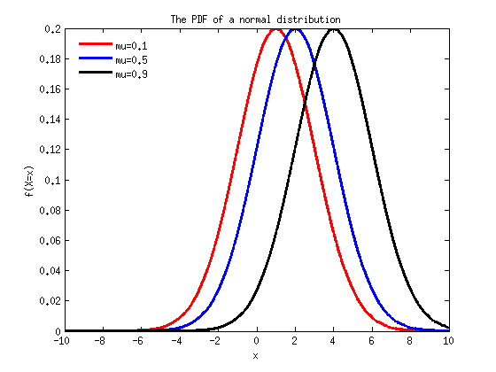
Do you notice that the shape of nomal distribution is bell? Also, the widths of the bells are the same, why? What is the PDF plot with fixed and varying ?
Assignments
Here goes the assignments for Lab 3.
Question 1. Plot the PDF and CDF for normal distribution with fixed  and varying
 ![$\sigma = [0.5, 1, 2]$](Lab3_eq19836.png) . Draw your observations with two to three sentences.
. Draw your observations with two to three sentences.
Question 2. Plot the PMF and CDF for geometric distribution with varying ![$p=[0.1, 0.5, 0.9]$](Lab3_eq22937.png) .
.
Submission. Put all of your code, figures, writeups in a single document with .doc or .docx or .pdf format. Submit the document through blackboard. Attention, .txt format is not acceptable.